Download this example

Download this example as a Jupyter Notebook or as a Python script.

---

PM synchronous motor transient analysis

This example shows how to use PyAEDT to create a Maxwell 2D transient analysis for an interior permanent magnet (PM) electric motor.

Model creation, setup and the solution process as well as visualization of the results are fully# automated. Only the motor cross-section is considered and 8-fold rotational symmetry is used to reduce the computational effort.

Keywords: Maxwell 2D, transient, motor.

Prerequisites

Perform imports

import csv
import tempfile
import time
from operator import attrgetter
from pathlib import Path

import ansys.aedt.core
import matplotlib.pyplot as plt
import numpy as np


from ansys.aedt.core.examples.downloads import download_file

Define constants

Constants help ensure consistency and avoid repetition throughout the example.

AEDT_VERSION = "2025.2"
NUM_CORES = 4
NG_MODE = False  # Open AEDT UI when it is launched.

Create temporary directory

Create a temporary working directory. The name of the working folder is stored in temp_folder.name.

Note: The final cell in the notebook cleans up the temporary folder. If you want to retrieve the AEDT project and data, do so before executing the final cell in the notebook.

temp_folder = tempfile.TemporaryDirectory(suffix=".ansys")

Model Preparation

Launch Maxwell 2D

Launch AEDT and Maxwell 2D after first setting up the project and design names, the solver, and the version. The following code also creates an instance of the Maxwell2d class named m2d.

project_name = Path(temp_folder.name) / "PM_Motor.aedt"
m2d = ansys.aedt.core.Maxwell2d(
    project=project_name,
    version=AEDT_VERSION,
    design="Sinusoidal",
    solution_type="TransientXY",
#    new_desktop=True,
    non_graphical=NG_MODE,
)
m2d.modeler.model_units = "mm"   # Specify model units

PyAEDT INFO: Python version 3.10.11 (tags/v3.10.11:7d4cc5a, Apr  5 2023, 00:38:17) [MSC v.1929 64 bit (AMD64)].
PyAEDT INFO: PyAEDT version 0.26.dev0.
PyAEDT INFO: Initializing Desktop session.
PyAEDT INFO: AEDT version 2025.2.
PyAEDT INFO: New AEDT session is starting on gRPC port 57871.
PyAEDT INFO: Starting new AEDT gRPC session on port 57871.
PyAEDT INFO: Launching AEDT server with gRPC transport mode: wnua
PyAEDT INFO: Electronics Desktop started on gRPC port 57871 after 10.8 seconds.
PyAEDT INFO: AEDT installation Path C:\Program Files\ANSYS Inc\v252\AnsysEM
PyAEDT INFO: Connected to AEDT gRPC session on port 57871.
PyAEDT WARNING: Service Pack is not detected. PyAEDT is currently connecting in Insecure Mode.
PyAEDT WARNING: Please download and install latest Service Pack to use connect to AEDT in Secure Mode.
PyAEDT INFO: Project PM_Motor has been created.
PyAEDT INFO: Added design 'Sinusoidal' of type Maxwell 2D.
PyAEDT INFO: AEDT objects correctly read
PyAEDT INFO: Modeler2D class has been initialized!
PyAEDT INFO: Modeler class has been initialized! Elapsed time: 0m 0sec

Define parameters

Initialize parameters to define the stator, rotor, and shaft geometric properties. The parameter names are consistent with those used in RMxprt.

Rotor geometric parameters:

geom_params = {
    "DiaGap": "132mm",
    "DiaStatorYoke": "198mm",
    "DiaStatorInner": "132mm",
    "DiaRotorLam": "130mm",
    "DiaShaft": "44.45mm",
    "DiaOuter": "198mm",
    "Airgap": "1mm",
    "SlotNumber": "48",
    "SlotType": "3",
}

Stator winding parameters:

wind_params = {
    "Layers": "1",
    "ParallelPaths": "2",
    "R_Phase": "7.5mOhm",
    "WdgExt_F": "5mm",
    "SpanExt": "30mm",
    "SegAngle": "0.25",
    "CoilPitch": "5",  # coil pitch in slots
    "Coil_SetBack": "3.605732823mm",
    "SlotWidth": "2.814mm",  # RMxprt Bs0
    "Coil_Edge_Short": "3.769235435mm",
    "Coil_Edge_Long": "15.37828521mm",
}

Additional model parameters:

mod_params = {
    "NumPoles": "8",                          # Number of poles
    "Model_Length": "80mm",                   # Motor length in the axial direction.
    "SymmetryFactor": "8",                    # Symmetry allows reduction of the model size.
    "Magnetic_Axial_Length": "150mm",
    "Stator_Lam_Length": "0mm",
    "StatorSkewAngle": "0deg",
    "NumTorquePointsPerCycle": "30",          # Number of points to sample torque during simulation.
    "mapping_angle": "0.125*4deg",
    "num_m": "16",
    "Section_Angle": "360deg/SymmetryFactor",  # Used to apply symmetry boundaries.
}

Stator current and initial rotor position

The motor will be driven by a sinusoidal current source that will apply values defined in the oper_params. The sources will be assigned to stator windings later in this example.

Sinusoidal current:

\[I_x = I_\text{peak} \cos\left(2\pi f t + \theta_i - \phi_x \right)\]

where \(x \in \{A, B, C\}\) is the electrical phase.

• \(I_x\rightarrow\) "IPeak" Amplitude of the current source for each winding.

• \(f \rightarrow\) "ElectricFrequency" Frequency of the current source.

• \(\theta_i\) "Theta_i" Initial rotor angle at \(t=0\).

• \(\phi_x\) is the phase angle. \(x=A\rightarrow 0^\circ, x=B\rightarrow120^\circ, x=C\rightarrow 240^\circ\).

oper_params = {
    "InitialPositionMD": "180deg/4",
    "IPeak": "480A",
    "MachineRPM": "3000rpm",
    "ElectricFrequency": "MachineRPM/60rpm*NumPoles/2*1Hz",
    "ElectricPeriod": "1/ElectricFrequency",
    "BandTicksinModel": "360deg/NumPoles/mapping_angle",
    "TimeStep": "ElectricPeriod/(2*BandTicksinModel)",
    "StopTime": "ElectricPeriod",
    "Theta_i": "135deg",
}

Update the Maxwell 2D model

Pass parameter names and values to the Maxwell 2D model.

for name, value in geom_params.items():
    m2d[name] = value
for name, value in wind_params.items():
    m2d[name] = value
for name, value in mod_params.items():
    m2d[name] = value
for name, value in oper_params.items():
    m2d[name] = value

Define materials and their properties.

First, download the \(B\)-\(H\) curves for the nonlinear magnetic materials from the example-data repository.

data_folder = Path(download_file(r'pyaedt/nissan', local_path=temp_folder.name))

Annealed copper at 65o C

mat_coils = m2d.materials.add_material("Copper (Annealed)_65C")
mat_coils.update()
mat_coils.conductivity = "49288048.9198"
mat_coils.permeability = "1"

PyAEDT INFO: Materials class has been initialized! Elapsed time: 0m 0sec
PyAEDT INFO: Adding new material to the Project Library: Copper (Annealed)_65C
PyAEDT INFO: Material has been added in Desktop.

Nonlinear magnetic materials

Define material properties.

The nonlinear \(B\)-\(H\) curves were retrieved from the example-data repository using the download_file() method.

The method bh_list() helps simplify assignment of data from the text file to the material permeability.

def bh_list(filepath):
    with open(filepath) as f:
        reader = csv.reader(f, delimiter="\t")                     # Ignore header
        next(reader)
        return [[float(row[0]), float(row[1])] for row in reader]  # Return a list of B,H values

Define the magnetic material properties.

The following image shows how the BH curve can be viewed in the AEDT user interface after the \(B\)-\(H\) curve has been assigned.

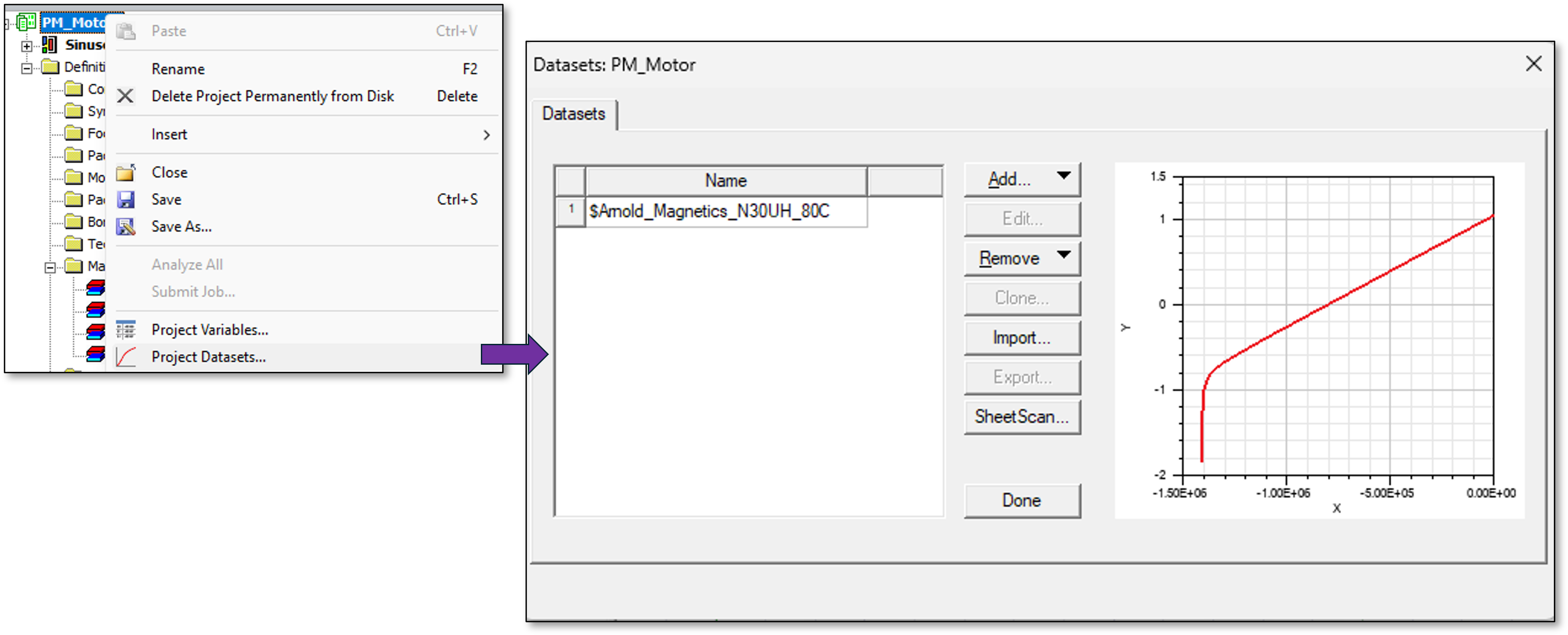
Define the material "Arnold_Magnetics_N30UH_80C".

mat_PM = m2d.materials.add_material(name="Arnold_Magnetics_N30UH_80C_new")
mat_PM.update()
mat_PM.conductivity = "555555.5556"
mat_PM.set_magnetic_coercivity(value=-800146.66287534, x=1, y=0, z=0)
mat_PM.mass_density = "7500"
mat_PM.permeability = bh_list(data_folder / 'BH_Arnold_Magnetics_N30UH_80C.tab')

PyAEDT INFO: Adding new material to the Project Library: Arnold_Magnetics_N30UH_80C_new
PyAEDT INFO: Material has been added in Desktop.

Define the laminate material, "30DH_20C_smooth".

mat_lam = m2d.materials.add_material("30DH_20C_smooth")
mat_lam.update()
mat_lam.conductivity = "1694915.25424"
kh = 71.7180985413
kc = 0.25092214579
ke = 12.1625774023
kdc = 0.001
eq_depth = 0.001
mat_lam.set_electrical_steel_coreloss(kh, kc, ke, kdc, eq_depth)
mat_lam.mass_density = "7650"
mat_lam.permeability = bh_list(data_folder / '30DH_20C_smooth.tab')

PyAEDT INFO: Adding new material to the Project Library: 30DH_20C_smooth
PyAEDT INFO: Material has been added in Desktop.

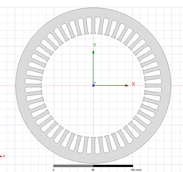
Create the stator

Create the geometry for the built-in user-defined primitive (UDP). A list of lists is created with the proper UDP parameters.

udp_par_list_stator = [
    ["DiaGap", "DiaGap"],
    ["DiaYoke", "DiaStatorYoke"],
    ["Length", "Stator_Lam_Length"],
    ["Skew", "StatorSkewAngle"],
    ["Slots", "SlotNumber"],
    ["SlotType", "SlotType"],
    ["Hs0", "1.2mm"],
    ["Hs01", "0mm"],
    ["Hs1", "0.4834227384999mm"],
    ["Hs2", "17.287669825502mm"],
    ["Bs0", "2.814mm"],
    ["Bs1", "4.71154109036mm"],
    ["Bs2", "6.9777285790998mm"],
    ["Rs", "2mm"],
    ["FilletType", "1"],
    ["HalfSlot", "0"],
    ["VentHoles", "0"],
    ["HoleDiaIn", "0mm"],
    ["HoleDiaOut", "0mm"],
    ["HoleLocIn", "0mm"],
    ["HoleLocOut", "0mm"],
    ["VentDucts", "0"],
    ["DuctWidth", "0mm"],
    ["DuctPitch", "0mm"],
    ["SegAngle", "0deg"],
    ["LenRegion", "Model_Length"],
    ["InfoCore", "0"],
]

stator = m2d.modeler.create_udp(
    dll="RMxprt/VentSlotCore.dll",
    parameters=udp_par_list_stator,
    library="syslib",
    name="my_stator",
)

Assign material and simulation properties to the stator. Additionally, the rendered color and "solve_inside" are set. The latter tells Maxwell to solve the full eddy-current solution inside the laminate conductors.

m2d.assign_material(assignment=stator, material="30DH_20C_smooth")
stator.name = "Stator"
stator.color = (0, 0, 255)  # rgb
stator.solve_inside = True

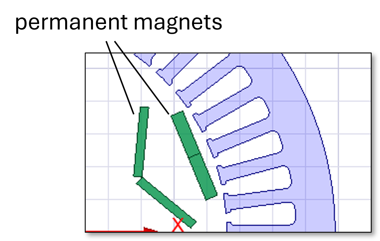
Create outer and inner permanent magnets

Draw permanent magnets.

IM1_points = [
    [56.70957112, 3.104886585, 0],
    [40.25081875, 16.67243502, 0],
    [38.59701538, 14.66621111, 0],
    [55.05576774, 1.098662669, 0],
]
OM1_points = [
    [54.37758185, 22.52393189, 0],
    [59.69688156, 9.68200639, 0],
    [63.26490432, 11.15992981, 0],
    [57.94560461, 24.00185531, 0],
]
IPM1 = m2d.modeler.create_polyline(
    points=IM1_points,
    cover_surface=True,
    name="PM_I1",
    material="Arnold_Magnetics_N30UH_80C_new",
)
IPM1.color = (0, 128, 64)
IPM1.solve_inside = True
OPM1 = m2d.modeler.create_polyline(
    points=OM1_points,
    cover_surface=True,
    name="PM_O1",
    material="Arnold_Magnetics_N30UH_80C_new",
)
OPM1.color = (0, 128, 64)
OPM1.solve_inside = True

Define the orientation for PM magnetization

The magnetization of the permanent magnets will be oriented along the \(x\)-direction of a local coordinate system associated with each magnet.

The method create_cs_magnets() will be used to create the coordinate system at the center of each magnet.

def create_magnet_cs(pm, cs_name, point_direction):
    """
    Parameters
    ----------
    pm : Polyline
        Permanent magnet 2D object.
    cs_name : str
        The name to be assigned to the coordinate system.
    point_direction : str
        "inner" B-field oriented toward the motor shaft.
        "outer" B-field oriented away from the shaft.
    """

    edges = sorted(pm.edges, key=attrgetter("length"), reverse=True)

    if point_direction == "outer":
        my_axis_pos = edges[0]
    elif point_direction == "inner":
        my_axis_pos = edges[1]

    m2d.modeler.create_face_coordinate_system(
        face=pm.faces[0],
        origin=pm.faces[0],
        axis_position=my_axis_pos,
        axis="X",
        name=cs_name,
    )
    pm.part_coordinate_system = cs_name
    m2d.modeler.set_working_coordinate_system("Global")

Create the coordinate system for PMs in the face center.

create_magnet_cs(IPM1, "CS_" + IPM1.name, "outer")
create_magnet_cs(OPM1, "CS_" + OPM1.name, "outer")

Duplicate and mirror PMs

Duplicate and mirror the magnets. Material definitions and the local coordinate systems are duplicated as well.

m2d.modeler.duplicate_and_mirror(
    assignment=[IPM1, OPM1],
    origin=[0, 0, 0],
    vector=[
        "cos((360deg/SymmetryFactor/2)+90deg)",
        "sin((360deg/SymmetryFactor/2)+90deg)",
        0,
    ],
)
id_PMs = m2d.modeler.get_objects_w_string(string_name="PM", case_sensitive=True)

The permanent magnets are shown below.

Create coils

coil = m2d.modeler.create_rectangle(
    origin=["DiaRotorLam/2+Airgap+Coil_SetBack", "-Coil_Edge_Short/2", 0],
    sizes=["Coil_Edge_Long", "Coil_Edge_Short", 0],
    name="Coil",
    material="Copper (Annealed)_65C",
)
coil.color = (255, 128, 0)
m2d.modeler.rotate(assignment=coil, axis="Z", angle="360deg/SlotNumber/2")
coil.duplicate_around_axis(
    axis="Z", angle="360deg/SlotNumber", clones="CoilPitch+1", create_new_objects=True
)
id_coils = m2d.modeler.get_objects_w_string(string_name="Coil", case_sensitive=True)

Create the shaft and surrounding region

region = m2d.modeler.create_circle(
    origin=[0, 0, 0],
    radius="DiaOuter/2",
    num_sides="SegAngle",
    is_covered=True,
    name="Region",
)
shaft = m2d.modeler.create_circle(
    origin=[0, 0, 0],
    radius="DiaShaft/2",
    num_sides="SegAngle",
    is_covered=True,
    name="Shaft",
)

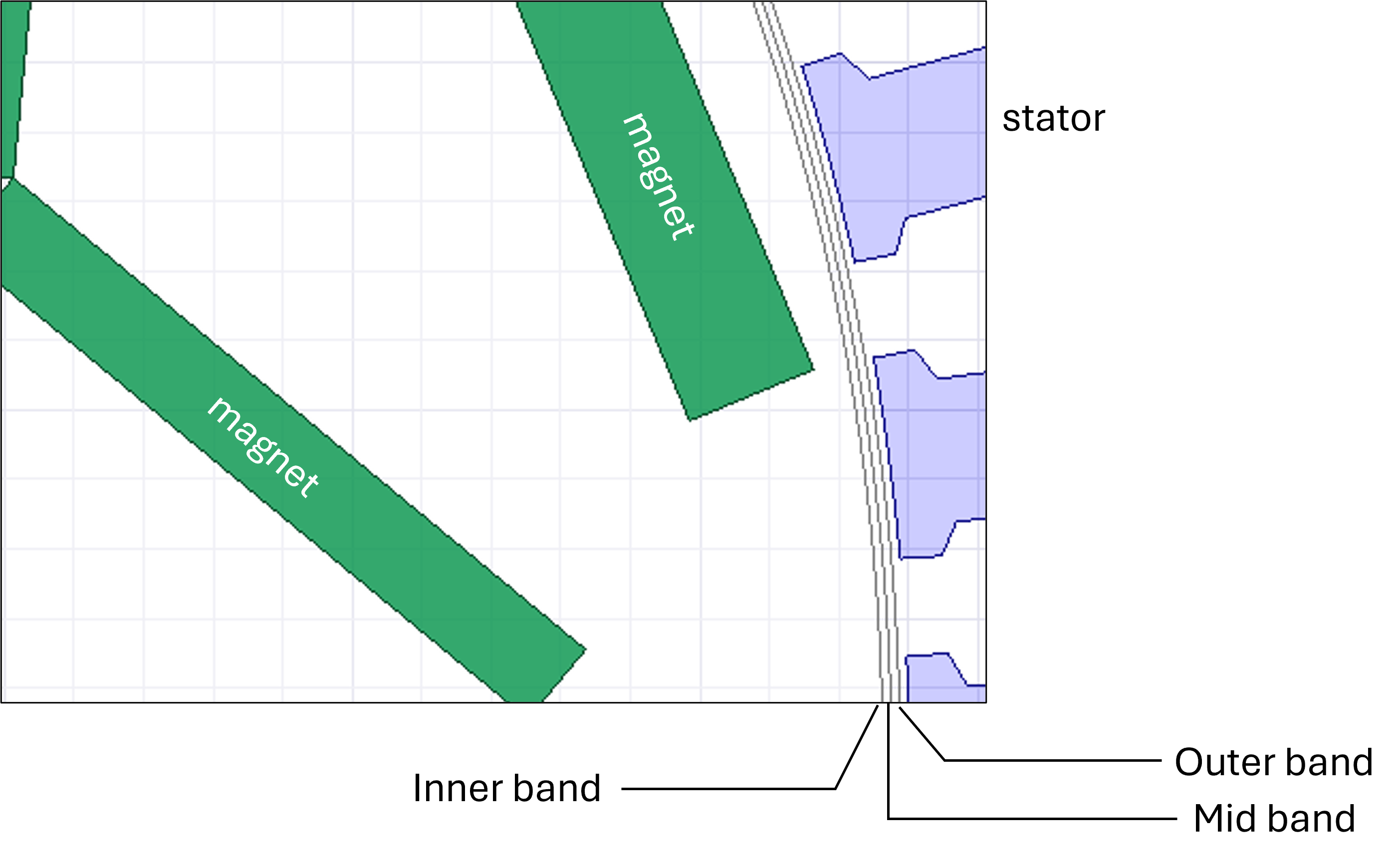
Create band objects

The band objects are required to assign the rotational motion of the machine. Everything outside the outer band object is stationary, while objects inside the band (i.e. the rotor and magnets) rotate.

Create the inner band, outer band, and outer band.

bandIN = m2d.modeler.create_circle(
    origin=[0, 0, 0],
    radius="(DiaGap - (1.5 * Airgap))/2",
    num_sides="mapping_angle",
    is_covered=True,
    name="Inner_Band",
)
bandMID = m2d.modeler.create_circle(
    origin=[0, 0, 0],
    radius="(DiaGap - (1.0 * Airgap))/2",
    num_sides="mapping_angle",
    is_covered=True,
    name="Band",
)
bandOUT= m2d.modeler.create_circle(
    origin=[0, 0, 0],
    radius="(DiaGap - (0.5 * Airgap))/2",
    num_sides="mapping_angle",
    is_covered=True,
    name="Outer_Band",
)

Assign “vacuum” material

The band objects, region and shaft will all be assigned the material “vacuum”.

vacuum_obj = [
    shaft,
    region,
    bandIN,
    bandMID,
    bandOUT,
]  # put shaft first
for item in vacuum_obj:
    item.color = (128, 255, 255)

Create rotor

Create the rotor with holes and pockets for the permanent magnets.

rotor = m2d.modeler.create_circle(
    origin=[0, 0, 0],
    radius="DiaRotorLam/2",
    num_sides=0,
    name="Rotor",
    material="30DH_20C_smooth",
)

rotor.color = (0, 128, 255)
rotor.solve_inside = True
m2d.modeler.subtract(blank_list=rotor, tool_list=shaft, keep_originals=True)
void_small_1 = m2d.modeler.create_circle(
    origin=[62, 0, 0], radius="2.55mm", num_sides=0, name="void1", material="vacuum"
)
void_small_1.solve_inside = True

m2d.modeler.duplicate_around_axis(
    assignment=void_small_1,
    axis="Z",
    angle="360deg/SymmetryFactor",
    clones=2,
    create_new_objects=False,
)

void_big_1 = m2d.modeler.create_circle(
    origin=[29.5643, 12.234389332712, 0],
    radius="9.88mm/2",
    num_sides=0,
    name="void_big",
    material="vacuum",
)
void_big_1.solve_inside = True

m2d.modeler.subtract(
    blank_list=rotor,
    tool_list=[void_small_1, void_big_1],
    keep_originals=False,
)

slot_IM1_points = [
    [37.5302872, 15.54555396, 0],
    [55.05576774, 1.098662669, 0],
    [57.33637589, 1.25, 0],
    [57.28982158, 2.626565019, 0],
    [40.25081875, 16.67243502, 0],
]
slot_OM1_points = [
    [54.37758185, 22.52393189, 0],
    [59.69688156, 9.68200639, 0],
    [63.53825619, 10.5, 0],
    [57.94560461, 24.00185531, 0],
]
slot_IM = m2d.modeler.create_polyline(
    points=slot_IM1_points, cover_surface=True, name="slot_IM1", material="vacuum"
)
slot_IM.solve_inside = True
slot_OM = m2d.modeler.create_polyline(
    points=slot_OM1_points, cover_surface=True, name="slot_OM1", material="vacuum"
)
slot_OM.solve_inside = True

m2d.modeler.duplicate_and_mirror(
    assignment=[slot_IM, slot_OM],
    origin=[0, 0, 0],
    vector=[
        "cos((360deg/SymmetryFactor/2)+90deg)",
        "sin((360deg/SymmetryFactor/2)+90deg)",
        0,
    ],
)

id_holes = m2d.modeler.get_objects_w_string(string_name="slot_", case_sensitive=True)
m2d.modeler.subtract(rotor, id_holes, keep_originals=True)

PyAEDT INFO: Parsing design objects. This operation can take time
PyAEDT INFO: Refreshing bodies from Object Info
PyAEDT INFO: Bodies Info Refreshed Elapsed time: 0m 0sec
PyAEDT INFO: 3D Modeler objects parsed. Elapsed time: 0m 0sec

True

Apply symmetry

Create a section of the machine for which electrical and geometric symmetry apply.

object_list = [stator, rotor] + vacuum_obj
m2d.modeler.create_coordinate_system(
    origin=[0, 0, 0],
    reference_cs="Global",
    name="Section",
    mode="axis",
    x_pointing=["cos(360deg/SymmetryFactor)", "sin(360deg/SymmetryFactor)", 0],
    y_pointing=["-sin(360deg/SymmetryFactor)", "cos(360deg/SymmetryFactor)", 0],
)

m2d.modeler.set_working_coordinate_system("Section")
m2d.modeler.split(assignment=object_list, plane="ZX", sides="NegativeOnly")
m2d.modeler.set_working_coordinate_system("Global")
m2d.modeler.split(assignment=object_list, plane="ZX", sides="PositiveOnly")

['Stator,Rotor,Shaft,Region,Inner_Band,Band,Outer_Band']

Create linked boundary conditions to apply electrical symmetry. Edges of the region object are selected based on their position. The edge selection point on the region object lies in the air-gap.

pos_1 = "((DiaGap - (1.0 * Airgap))/4)"
id_bc_1 = m2d.modeler.get_edgeid_from_position(
    position=[pos_1, 0, 0], assignment="Region"
)
id_bc_2 = m2d.modeler.get_edgeid_from_position(
    position=[
        pos_1 + "*cos((360deg/SymmetryFactor))",
        pos_1 + "*sin((360deg/SymmetryFactor))",
        0,
    ],
    assignment="Region",
)
m2d.assign_master_slave(
    independent=id_bc_1,
    dependent=id_bc_2,
    reverse_master=False,
    reverse_slave=True,
    same_as_master=False,
    boundary="Matching",
)

PyAEDT INFO: Boundary Independent Matching has been created.
PyAEDT INFO: Boundary Dependent Matching_dep has been created.

(Matching, Matching_dep)

Assign outer boundary condition

Assign the boundary condition for the magnetic vector potnetial, \(A_z=0\) on the outer perimeter of the motor.

pos_2 = "(DiaOuter/2)"
id_bc_az = m2d.modeler.get_edgeid_from_position(
    position=[
        pos_2 + "*cos((360deg/SymmetryFactor/2))",
        pos_2 + "*sin((360deg/SymmetryFactor)/2)",
        0,
    ],
    assignment="Region",
)
m2d.assign_vector_potential(
    assignment=id_bc_az, vector_value=0, boundary="VectorPotentialZero"
)

PyAEDT INFO: Boundary Vector Potential VectorPotentialZero has been created.

VectorPotentialZero

Define stator winding current sources

The stator windings will be driven with a 3-phase sinusoidal current whose amplitude and frequency were defined earlier parameters that were defined earlier in this example. The windigs have 6 conductors each. The following function can be used define the windings and assign excitations:

def assign_winding(name="A", phase="", obj_p=None, obj_n=None, nconductors=6):
    """
    Parameters
    ----------
    phase : str, Optinonal
        Current source phase. For example, "120deg"
    obj_p : str
        The name of the winding object for positive current injection.
    obj_n : str
        The name of the winding object where current returns.
    nconductors : int
        Number of strands per winding.
    name : str
        String to use for naming sources and windings.

    """
    phase_str = f"+ Theta_i - {phase}"
    ph_current = f"IPeak * cos(2*pi*ElectricFrequency*time {phase_str})"
    phase_name = f"Phase_{name}"
    pos_coil_name = f"Phase_{name}_pos"
    neg_coil_name = f"Phase_{name}_neg"
    m2d.assign_coil(
        assignment=[obj_p],
        conductors_number=nconductors,
        polarity="Positive",
        name=pos_coil_name,
        )
    m2d.assign_coil(
        assignment=[obj_n],
        conductors_number=nconductors,
        polarity="Negative",
        name=neg_coil_name,
        )
    m2d.assign_winding(
        assignment=None,
        winding_type="Current",
        is_solid=False,
        current=ph_current,
        parallel_branches=1,
        name=phase_name,
        )
    m2d.add_winding_coils(
        assignment=phase_name, coils=[pos_coil_name, neg_coil_name]
)

assign_winding("A", "0deg", "Coil", "Coil_5")
assign_winding("B", "120deg", "Coil_3", "Coil_4")
assign_winding("C", "240deg", "Coil_1", "Coil_2")

PyAEDT INFO: Boundary Coil Phase_A_pos has been created.
PyAEDT INFO: Boundary Coil Phase_A_neg has been created.
PyAEDT INFO: Boundary Winding Phase_A has been created.
PyAEDT INFO: Boundary Coil Phase_B_pos has been created.
PyAEDT INFO: Boundary Coil Phase_B_neg has been created.
PyAEDT INFO: Boundary Winding Phase_B has been created.
PyAEDT INFO: Boundary Coil Phase_C_pos has been created.
PyAEDT INFO: Boundary Coil Phase_C_neg has been created.
PyAEDT INFO: Boundary Winding Phase_C has been created.

Set the \(J_z=0\) on the permanent magnets.

PM_list = id_PMs
for item in PM_list:
    m2d.assign_current(assignment=item, amplitude=0, solid=True, name=item + "_I0")

PyAEDT INFO: Boundary Current PM_I1_I0 has been created.
PyAEDT INFO: Boundary Current PM_O1_I0 has been created.
PyAEDT INFO: Boundary Current PM_I1_1_I0 has been created.
PyAEDT INFO: Boundary Current PM_O1_1_I0 has been created.

Create mesh operations

Mesh operations are used to refine the finite element mesh and ensure accuracy of the solution. This example uses a relatively coarse mesh so the simulation runs quickly. Accuracy can be improved by increasing mesh density (reducing maximum_length).

m2d.mesh.assign_length_mesh(     # Coils
    assignment=id_coils,
    inside_selection=True,
    maximum_length=3,
    maximum_elements=None,
    name="coils",
)
m2d.mesh.assign_length_mesh(      # Stator
    assignment=stator,
    inside_selection=True,
    maximum_length=3,
    maximum_elements=None,
    name="stator",
)
m2d.mesh.assign_length_mesh(      # Rotor
    assignment=rotor,
    inside_selection=True,
    maximum_length=3,
    maximum_elements=None,
    name="rotor",
)

PyAEDT INFO: Mesh class has been initialized! Elapsed time: 0m 0sec
PyAEDT INFO: Mesh class has been initialized! Elapsed time: 0m 0sec

rotor

Enable core loss calculation

core_loss_list = ["Rotor", "Stator"]
m2d.set_core_losses(core_loss_list, core_loss_on_field=True)

True

Enable calcuation of the time-dependent inductance

m2d.change_inductance_computation(
    compute_transient_inductance=True, incremental_matrix=False
)

True

Specify the length of the motor.

The motor length along with rotor mass are used to calculate the interia for the transient simulation.

m2d.model_depth = "Magnetic_Axial_Length"

Specify the symmetry multiplier

m2d.change_symmetry_multiplier("SymmetryFactor")

True

Assign motion setup to object

Assign a motion setup to a Band object named RotatingBand_mid.

m2d.assign_rotate_motion(
    assignment="Band",
    coordinate_system="Global",
    axis="Z",
    positive_movement=True,
    start_position="InitialPositionMD",
    angular_velocity="MachineRPM",
)

PyAEDT INFO: Boundary Band MotionSetup1 has been created.

MotionSetup1

Create simulation setup

setup_name = "MySetupAuto"
setup = m2d.create_setup(name=setup_name)
setup.props["StopTime"] = "StopTime"
setup.props["TimeStep"] = "TimeStep"
setup.props["SaveFieldsType"] = "None"
setup.props["OutputPerObjectCoreLoss"] = True
setup.props["OutputPerObjectSolidLoss"] = True
setup.props["OutputError"] = True
setup.update()
m2d.validate_simple()  # Validate the model

model = m2d.plot(show=False)
model.plot(Path(temp_folder.name) / "Image.jpg")

PyAEDT INFO: Parsing C:\Users\ansys\AppData\Local\Temp\tmp46hxp4y4.ansys\PM_Motor.aedt.
PyAEDT INFO: File C:\Users\ansys\AppData\Local\Temp\tmp46hxp4y4.ansys\PM_Motor.aedt correctly loaded. Elapsed time: 0m 0sec
PyAEDT INFO: aedt file load time 0.003516674041748047
PyAEDT INFO: PostProcessor class has been initialized! Elapsed time: 0m 0sec
PyAEDT INFO: PostProcessor class has been initialized! Elapsed time: 0m 0sec
PyAEDT INFO: Post class has been initialized! Elapsed time: 0m 0sec

True

Initialize definitions for output variables

Initialize the definitions for the output variables. These are used later to generate reports.

output_vars = {
    "Current_A": "InputCurrent(Phase_A)",
    "Current_B": "InputCurrent(Phase_B)",
    "Current_C": "InputCurrent(Phase_C)",
    "Flux_A": "FluxLinkage(Phase_A)",
    "Flux_B": "FluxLinkage(Phase_B)",
    "Flux_C": "FluxLinkage(Phase_C)",
    "pos": "(Moving1.Position -InitialPositionMD) *NumPoles/2",
    "cos0": "cos(pos)",
    "cos1": "cos(pos-2*PI/3)",
    "cos2": "cos(pos-4*PI/3)",
    "sin0": "sin(pos)",
    "sin1": "sin(pos-2*PI/3)",
    "sin2": "sin(pos-4*PI/3)",
    "Flux_d": "2/3*(Flux_A*cos0+Flux_B*cos1+Flux_C*cos2)",
    "Flux_q": "-2/3*(Flux_A*sin0+Flux_B*sin1+Flux_C*sin2)",
    "I_d": "2/3*(Current_A*cos0 + Current_B*cos1 + Current_C*cos2)",
    "I_q": "-2/3*(Current_A*sin0 + Current_B*sin1 + Current_C*sin2)",
    "Irms": "sqrt(I_d^2+I_q^2)/sqrt(2)",
    "ArmatureOhmicLoss_DC": "Irms^2*R_phase",
    "Lad": "L(Phase_A,Phase_A)*cos0 + L(Phase_A,Phase_B)*cos1 + L(Phase_A,Phase_C)*cos2",
    "Laq": "L(Phase_A,Phase_A)*sin0 + L(Phase_A,Phase_B)*sin1 + L(Phase_A,Phase_C)*sin2",
    "Lbd": "L(Phase_B,Phase_A)*cos0 + L(Phase_B,Phase_B)*cos1 + L(Phase_B,Phase_C)*cos2",
    "Lbq": "L(Phase_B,Phase_A)*sin0 + L(Phase_B,Phase_B)*sin1 + L(Phase_B,Phase_C)*sin2",
    "Lcd": "L(Phase_C,Phase_A)*cos0 + L(Phase_C,Phase_B)*cos1 + L(Phase_C,Phase_C)*cos2",
    "Lcq": "L(Phase_C,Phase_A)*sin0 + L(Phase_C,Phase_B)*sin1 + L(Phase_C,Phase_C)*sin2",
    "L_d": "(Lad*cos0 + Lbd*cos1 + Lcd*cos2) * 2/3",
    "L_q": "(Laq*sin0 + Lbq*sin1 + Lcq*sin2) * 2/3",
    "OutputPower": "Moving1.Speed*Moving1.Torque",
    "Ui_A": "InducedVoltage(Phase_A)",
    "Ui_B": "InducedVoltage(Phase_B)",
    "Ui_C": "InducedVoltage(Phase_C)",
    "Ui_d": "2/3*(Ui_A*cos0 + Ui_B*cos1 + Ui_C*cos2)",
    "Ui_q": "-2/3*(Ui_A*sin0 + Ui_B*sin1 + Ui_C*sin2)",
    "U_A": "Ui_A+R_Phase*Current_A",
    "U_B": "Ui_B+R_Phase*Current_B",
    "U_C": "Ui_C+R_Phase*Current_C",
    "U_d": "2/3*(U_A*cos0 + U_B*cos1 + U_C*cos2)",
    "U_q": "-2/3*(U_A*sin0 + U_B*sin1 + U_C*sin2)",
}

Create output variables for postprocessing

for k, v in output_vars.items():
    m2d.create_output_variable(k, v)

Create reports

Define common keyword arguments shared by all time-domain reports, then create each report by specifying only its expressions and plot name. This avoids repeating the same arguments for every create_report call.

report_kwargs = dict(
    setup_sweep_name=m2d.nominal_sweep,
    domain="Sweep",
    primary_sweep_variable="Time",
    plot_type="Rectangular Plot",
)

reports = [
    ("Moving1.Torque",                                                                      "TorquePlots"),
    (["U_A", "U_B", "U_C", "Ui_A", "Ui_B", "Ui_C"],                                       "PhaseVoltages"),
    (["CoreLoss", "SolidLoss", "ArmatureOhmicLoss_DC"],                                     "Losses"),
    (["InputCurrent(Phase_A)", "InputCurrent(Phase_B)", "InputCurrent(Phase_C)"],           "PhaseCurrents"),
    (["FluxLinkage(Phase_A)", "FluxLinkage(Phase_B)", "FluxLinkage(Phase_C)"],              "PhaseFluxes"),
    (["I_d", "I_q"],                                                                        "Currents_dq"),
    (["Flux_d", "Flux_q"],                                                                  "Fluxes_dq"),
    (["Ui_d", "Ui_q"],                                                                      "InducedVoltages_dq"),
    (["U_d", "U_q"],                                                                        "Voltages_dq"),
    (["L(Phase_A,Phase_A)", "L(Phase_B,Phase_B)", "L(Phase_C,Phase_C)",
      "L(Phase_A,Phase_B)", "L(Phase_A,Phase_C)", "L(Phase_B,Phase_C)"],                   "PhaseInductances"),
    (["L_d", "L_q"],                                                                        "Inductances_dq"),
    (["CoreLoss", "CoreLoss(Stator)", "CoreLoss(Rotor)"],                                   "CoreLosses"),
    (["EddyCurrentLoss", "EddyCurrentLoss(Stator)", "EddyCurrentLoss(Rotor)"],             "EddyCurrentLosses (Core)"),
    (["ExcessLoss", "ExcessLoss(Stator)", "ExcessLoss(Rotor)"],                             "ExcessLosses (Core)"),
    (["HysteresisLoss", "HysteresisLoss(Stator)", "HysteresisLoss(Rotor)"],                "HysteresisLosses (Core)"),
    (["SolidLoss", "SolidLoss(IPM1)", "SolidLoss(IPM1_1)", "SolidLoss(OPM1)", "SolidLoss(OPM1_1)"], "SolidLoss"),
]

for expressions, plot_name in reports:
    m2d.post.create_report(expressions=expressions, plot_name=plot_name, **report_kwargs)

PyAEDT WARNING: No report category provided. Automatically identified Transient
PyAEDT WARNING: No report category provided. Automatically identified Transient
PyAEDT WARNING: No report category provided. Automatically identified Transient
PyAEDT WARNING: No report category provided. Automatically identified Transient
PyAEDT WARNING: No report category provided. Automatically identified Transient
PyAEDT WARNING: No report category provided. Automatically identified Transient
PyAEDT WARNING: No report category provided. Automatically identified Transient
PyAEDT WARNING: No report category provided. Automatically identified Transient
PyAEDT WARNING: No report category provided. Automatically identified Transient
PyAEDT WARNING: No report category provided. Automatically identified Transient

Analyze and save project

m2d.save_project()
m2d.analyze_setup(setup_name, use_auto_settings=False, cores=NUM_CORES)

PyAEDT INFO: Project PM_Motor Saved correctly
PyAEDT INFO: Key Desktop/ActiveDSOConfigurations/Maxwell 2D correctly changed.
PyAEDT INFO: Solving design setup MySetupAuto
PyAEDT INFO: Design setup MySetupAuto solved correctly in 0.0h 2.0m 8.0s
PyAEDT INFO: Key Desktop/ActiveDSOConfigurations/Maxwell 2D correctly changed.

True

Create flux lines plot on region

Create a flux lines plot on a region. The object_list is formerly created when the section is applied.

faces_reg = m2d.modeler.get_object_faces(object_list[1].name)  # Region
plot1 = m2d.post.create_fieldplot_surface(
    assignment=faces_reg,
    quantity="Flux_Lines",
    intrinsics={"Time": m2d.variable_manager.variables["StopTime"].evaluated_value},
    plot_name="Flux_Lines",
)

PyAEDT INFO: Active Design set to Sinusoidal

Export a field plot to an image file

Export the flux lines plot to an image file using Python PyVista.

m2d.post.plot_field_from_fieldplot(plot1.name, show=False)

Class: ansys.aedt.core.visualization.plot.pyvista.ModelPlotter

Get solution data

Retrieve shaft torque as a function of time. get_expression_data returns the time axis (in ns) and the torque values as numpy arrays in a single call.

solutions = m2d.post.get_solution_data(
    expressions="Moving1.Torque",
    setup_sweep_name=m2d.nominal_sweep,
    primary_sweep_variable="Time",
    domain="Sweep",
)

PyAEDT WARNING: No report category provided. Automatically identified Transient
PyAEDT INFO: Solution Data Correctly Loaded.
Time to initialize solution data:0.08845138549804688
Time to initialize solution data:0.08845138549804688

time_ns, torque = solutions.get_expression_data(formula="real")
avg_torque = np.mean(torque)

Export a report to a file

Export 2D plot data to a CSV file.

m2d.post.export_report_to_file(
    output_dir=temp_folder.name, plot_name="TorquePlots", extension=".csv"
)

'C:\\Users\\ansys\\AppData\\Local\\Temp\\tmp46hxp4y4.ansys\\TorquePlots.csv'

Plot torque over the second quarter of the electric period

Extract and plot torque values from ElectricPeriod/4 to ElectricPeriod/2. The electric period is retrieved from the design variables in seconds and converted to nanoseconds to match the time axis units returned by get_expression_data.

ep_ns = m2d.variable_manager.design_variables["ElectricPeriod"].numeric_value * 1e9
mask = (time_ns >= ep_ns / 4) & (time_ns <= ep_ns / 2)

fig, ax = plt.subplots()
ax.plot(time_ns[mask], torque[mask], marker="o")
ax.set_xlabel("Time (ns)")
ax.set_ylabel("Torque (N·m)")
ax.set_title("Torque vs Time (Quarter to Half Period)")

Text(0.5, 1.0, 'Torque vs Time (Quarter to Half Period)')

Uncomment the following line to display the matplotlib plot: plt.show()

Finish

Save the project

m2d.save_project()
m2d.release_desktop()
# Wait 3 seconds to allow AEDT to shut down before cleaning the temporary directory.
time.sleep(3)

PyAEDT INFO: Project PM_Motor Saved correctly
PyAEDT INFO: Desktop has been released and closed.

Clean up

All project files are saved in the folder temp_folder.name. If you’ve run this example as a Jupyter notebook, you can retrieve those project files. The following cell removes all temporary files, including the project folder.

temp_folder.cleanup()

---

Download this example

Download this example as a Jupyter Notebook or as a Python script.