Download this example

Download this example as a Jupyter Notebook or as a Python script.

---

Component antenna array

This example shows how to create an antenna array using 3D components for the unit cell definition. You will see how to set up the analysis, generates the EM solution, and post-process the solution data using Matplotlib and PyVista. This example runs only on Windows using CPython.

Keywords: HFSS, antenna array, 3D components, far field.

Prerequisites

Perform imports

import os
import tempfile
import time

from ansys.aedt.core import Hfss
from ansys.aedt.core.visualization.advanced.farfield_visualization import \
    FfdSolutionData
from ansys.aedt.core.downloads import download_3dcomponent
from ansys.aedt.core.generic import file_utils

Define constants

Constants help ensure consistency and avoid repetition throughout the example.

AEDT_VERSION = "2025.1"
NUM_CORES = 4
NG_MODE = False  # Open AEDT UI when it is launched.

Create temporary directory

Create a temporary working directory. The name of the working folder is stored in temp_folder.name.

Note: The final cell in the notebook cleans up the temporary folder. If you want to retrieve the AEDT project and data, do so before executing the final cell in the notebook.

temp_folder = tempfile.TemporaryDirectory(suffix=".ansys")

Download 3D component

Download the 3D component that will be used to define the unit cell in the antenna array.

path_to_3dcomp = download_3dcomponent(destination=temp_folder.name)

Launch HFSS

The following cell creates a new Hfss object. Electronics desktop is launched and a new HFSS design is inserted into the project.

project_name = os.path.join(temp_folder.name, "array.aedt")
hfss = Hfss(
    project=project_name,
    version=AEDT_VERSION,
    design="Array_Simple",
    non_graphical=NG_MODE,
    new_desktop=False,  # Set to `False` to connect to an existing AEDT session.
)

print("Project name " + project_name)

PyAEDT INFO: Python version 3.10.11 (tags/v3.10.11:7d4cc5a, Apr  5 2023, 00:38:17) [MSC v.1929 64 bit (AMD64)].
PyAEDT INFO: PyAEDT version 0.16.dev0.
PyAEDT INFO: Initializing new Desktop session.
PyAEDT INFO: Log on console is enabled.
PyAEDT INFO: Log on file C:\Users\ansys\AppData\Local\Temp\pyaedt_ansys_ad1b7389-3294-4be6-abc2-f076039f7814.log is enabled.
PyAEDT INFO: Log on AEDT is disabled.
PyAEDT INFO: Debug logger is disabled. PyAEDT methods will not be logged.
PyAEDT INFO: Launching PyAEDT with gRPC plugin.
PyAEDT INFO: New AEDT session is starting on gRPC port 50016.
PyAEDT INFO: Electronics Desktop started on gRPC port: 50016 after 7.0052268505096436 seconds.
PyAEDT INFO: AEDT installation Path C:\Program Files\ANSYS Inc\v251\AnsysEM
PyAEDT INFO: Ansoft.ElectronicsDesktop.2025.1 version started with process ID 9452.
PyAEDT INFO: Project array has been created.
PyAEDT INFO: Added design 'Array_Simple' of type HFSS.
PyAEDT INFO: Aedt Objects correctly read
Project name C:\Users\ansys\AppData\Local\Temp\tmpve8w9etd.ansys\array.aedt

Read array definition

Read array definition from the JSON file.

array_definition = file_utils.read_json(
    os.path.join(path_to_3dcomp, "array_simple.json")
)

Add the 3D component definition

The JSON file links the unit cell to the 3D component named “Circ_Patch_5GHz1”. This can be seen by examining array_definition["cells"]. The following code prints the row and column indices of the array elements along with the name of the 3D component for each element.

Note: The array_definition["cells"] is of type dict and the key is builta as a string from the (row, column) indices of the array element. For example: the key for the element in the first row and 2nd column is "(1,2)".

print("Element\t\tName")
print("--------\t-------------")
for cell in array_definition["cells"]:
    cell_name = array_definition["cells"][cell]["name"]
    print(f"{cell}\t\t'{cell_name}'.")

Element         Name
--------        -------------
(1,1)           'Circ_Patch_5GHz1'.
(1,2)           'Circ_Patch_5GHz1'.
(1,3)           'Circ_Patch_5GHz1'.
(2,1)           'Circ_Patch_5GHz1'.
(2,2)           'Circ_Patch_5GHz1'.
(2,3)           'Circ_Patch_5GHz1'.
(3,1)           'Circ_Patch_5GHz1'.
(3,2)           'Circ_Patch_5GHz1'.
(3,3)           'Circ_Patch_5GHz1'.

Each unit cell is defined by a 3D Component. The 3D component may be added to the HFSS design using the method [Hfss.modeler.insert_3d_component()] (https://aedt.docs.pyansys.com/version/stable/API/_autosummary/ansys.aedt.core.modeler.modeler_3d.Modeler3D.insert_3d_component.html) or it can be added as a key to the array_definition as shown below.

array_definition["Circ_Patch_5GHz1"] = os.path.join(path_to_3dcomp, "Circ_Patch_5GHz.a3dcomp")

Note that the 3D component name is identical to the value for each element in the "cells" dictionary. For example, ``array_definition[“cells”][0][0][“name”]

Create the 3D component array in HFSS

The array is now generated in HFSS from the information in array_definition. If a 3D component is not available in the design, it is loaded into the dictionary from the path that you specify. The following code edits the dictionary to point to the location of the A3DCOMP file.

array = hfss.add_3d_component_array_from_json(array_definition, name="circ_patch_array")

PyAEDT INFO: Modeler class has been initialized! Elapsed time: 0m 0sec
PyAEDT INFO: Parsing C:/Users/ansys/AppData/Local/Temp/tmpve8w9etd.ansys/array.aedt.
PyAEDT INFO: File C:/Users/ansys/AppData/Local/Temp/tmpve8w9etd.ansys/array.aedt correctly loaded. Elapsed time: 0m 0sec
PyAEDT INFO: aedt file load time 0.016784191131591797
PyAEDT INFO: Project array Saved correctly
PyAEDT INFO: Parsing C:/Users/ansys/AppData/Local/Temp/tmpve8w9etd.ansys/array.aedt.
PyAEDT INFO: File C:/Users/ansys/AppData/Local/Temp/tmpve8w9etd.ansys/array.aedt correctly loaded. Elapsed time: 0m 0sec
PyAEDT INFO: aedt file load time 0.09501457214355469

Modify cells

Make the center element passive and rotate the corner elements.

array.cells[1][1].is_active = False
array.cells[0][0].rotation = 90
array.cells[0][2].rotation = 90
array.cells[2][0].rotation = 90
array.cells[2][2].rotation = 90

Set up simulation and run analysis

Set up a simulation and analyze it.

setup = hfss.create_setup()
setup.props["Frequency"] = "5GHz"
setup.props["MaximumPasses"] = 3
hfss.analyze(cores=NUM_CORES)

PyAEDT INFO: Key Desktop/ActiveDSOConfigurations/HFSS correctly changed.
PyAEDT INFO: Solving all design setups.
PyAEDT INFO: Key Desktop/ActiveDSOConfigurations/HFSS correctly changed.
PyAEDT INFO: Design setup None solved correctly in 0.0h 0.0m 42.0s

True

Postprocess

Retrieve far-field data

Get far-field data. After the simulation completes, the far field data is generated port by port and stored in a data class.

ffdata = hfss.get_antenna_data(setup=hfss.nominal_adaptive, sphere="Infinite Sphere1")

PyAEDT INFO: Far field sphere Infinite Sphere1 is created.
PyAEDT INFO: PostProcessor class has been initialized! Elapsed time: 0m 0sec
PyAEDT INFO: Post class has been initialized! Elapsed time: 0m 0sec
PyAEDT INFO: Solution Data Correctly Loaded.
PyAEDT INFO: Exporting antenna metadata...
PyAEDT INFO: Antenna metadata exported.
PyAEDT INFO: Exporting geometry...
PyAEDT INFO: Exporting embedded element patterns.... Done: 2.092064380645752 seconds

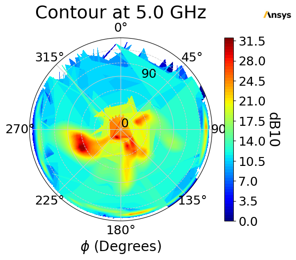
Generate contour plot

Generate a contour plot. You can define the Theta scan and Phi scan.

ffdata.farfield_data.plot_contour(
    quantity="RealizedGain",
    title=f"Contour at {ffdata.farfield_data.frequency * 1E-9:0.1f} GHz"
)

<ansys.aedt.core.visualization.plot.matplotlib.ReportPlotter at 0x1d7214d99c0>

Save the project and data

Farfield data can be accessed from disk after the solution has been generated using the metadata_file property of ffdata.

metadata_file = ffdata.metadata_file
working_directory = hfss.working_directory

hfss.save_project()
hfss.release_desktop()
# Wait 3 seconds to allow AEDT to shut down before cleaning the temporary directory.
time.sleep(3)

PyAEDT INFO: Project array Saved correctly
PyAEDT INFO: Desktop has been released and closed.

Load far field data

An instance of the FfdSolutionData class can be instantiated from the metadata file. Embedded element patters are linked through the metadata file.

ffdata = FfdSolutionData(input_file=metadata_file)

Generate contour plot

Generate a contour plot. You can define the Theta scan and Phi scan.

ffdata.plot_contour(
    quantity="RealizedGain", title=f"Contour at {ffdata.frequency * 1e-9:.1f} GHz"
)

<ansys.aedt.core.visualization.plot.matplotlib.ReportPlotter at 0x1d721cada20>

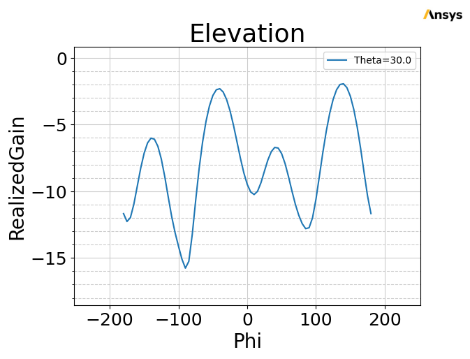
Generate 2D cutout plots

Generate 2D cutout plots. You can define the Theta scan and Phi scan.

ffdata.plot_cut(
    quantity="RealizedGain",
    primary_sweep="theta",
    secondary_sweep_value=[-180, -75, 75],
    title=f"Azimuth at {ffdata.frequency * 1E-9:.1f} GHz",
    quantity_format="dB10",
)

ffdata.plot_cut(
    quantity="RealizedGain",
    primary_sweep="phi",
    secondary_sweep_value=30,
    title="Elevation",
    quantity_format="dB10",
)

<ansys.aedt.core.visualization.plot.matplotlib.ReportPlotter at 0x1d723b3ead0>

Generate 3D plot

Generate 3D plots. You can define the Theta scan and Phi scan.

ffdata.plot_3d(
    quantity="RealizedGain",
    output_file=os.path.join(working_directory, "Image.jpg"),
    show=False,
)

C:\actions-runner\_work\pyaedt-examples\pyaedt-examples\.venv\lib\site-packages\pyvista\jupyter\notebook.py:37: UserWarning: Failed to use notebook backend:

No module named 'trame'

Falling back to a static output.
  warnings.warn(

<pyvista.plotting.plotter.Plotter at 0x1d723b73c40>

Clean up

All project files are saved in the folder temp_folder.name. If you’ve run this example as a Jupyter notebook, you can retrieve those project files. The following cell removes all temporary files, including the project folder.

temp_folder.cleanup()

---

Download this example

Download this example as a Jupyter Notebook or as a Python script.