Download this example
Download this example as a Jupyter Notebook or as a Python script.
Dipole antenna#
This example demonstrates how to create and analyze a half-wave dipole antenna in HFSS.
Keywords: HFSS, antenna, 3D component, far field.
Prerequisites#
Perform imports#
Import the packages required to run this example.
[1]:
import os
import tempfile
import time

from ansys.aedt.core import Hfss
Define constants#
Constants help ensure consistency and avoid repetition throughout the example.
[2]:
AEDT_VERSION = "2026.1"
NUM_CORES = 4
NG_MODE = True  # Open AEDT UI when it is launched.
Create temporary directory#
Create a temporary working directory. The name of the working folder is stored in temp_folder.name.
Note: The final cell in this notebook cleans up the temporary folder. If you want to retrieve the AEDT project and data, do so before executing the final cell in the notebook.
[3]:
temp_folder = tempfile.TemporaryDirectory(suffix=".ansys")
Launch HFSS#
Create an instance of the Hfss class. The Ansys Electronics Desktop will be launched with an active HFSS design. The hfss object is subsequently used to create and simulate the dipole antenna.
[4]:
project_name = os.path.join(temp_folder.name, "dipole.aedt")
hfss = Hfss(
    version=AEDT_VERSION,
    non_graphical=NG_MODE,
    project=project_name,
    new_desktop=True,
    solution_type="Modal",
)
PyAEDT INFO: Python version 3.10.11 (tags/v3.10.11:7d4cc5a, Apr  5 2023, 00:38:17) [MSC v.1929 64 bit (AMD64)].
PyAEDT INFO: PyAEDT version 1.3.dev0.
PyAEDT INFO: Initializing new Desktop session.
PyAEDT INFO: AEDT version 2026.1.
PyAEDT INFO: New AEDT session is starting on gRPC port 56608.
PyAEDT INFO: Starting new AEDT gRPC session on port 56608.
PyAEDT INFO: Launching AEDT server with gRPC transport mode: wnua
PyAEDT INFO: Electronics Desktop started on gRPC port 56608 after 10.2 seconds.
PyAEDT INFO: AEDT installation Path C:\Program Files\ANSYS Inc\v261\AnsysEM
PyAEDT INFO: 2026.1 version started with process ID 5088.
PyAEDT INFO: Non-graphical mode detected. Disabling Desktop logs.
PyAEDT INFO: Project dipole has been created.
PyAEDT INFO: No design is present. Inserting a new design.
PyAEDT INFO: Added design 'HFSS_VMY' of type HFSS.
PyAEDT INFO: AEDT objects correctly read
Model Preparation#
Define the dipole length as a parameter#
The dipole length can be modified by changing the parameter l_dipole to tune the resonance frequency.
The dipole will nominally be resonant at the half-wavelength frequency:
[5]:
hfss["l_dipole"] = "10.2cm"
component_name = "Dipole_Antenna_DM"
freq_range = ["1GHz", "2GHz"]  # Frequency range for analysis and post-processing.
center_freq = "1.5GHz"  # Center frequency
freq_step = "0.5GHz"
Insert the dipole antenna model#
The 3D component “Dipole_Antenna_DM” will be inserted from the built-in syslib folder. The full path to the 3D components can be retrieved from hfss.components3d.
The component is inserted using the method hfss.modeler.insert_3d_component().
The first argument passed to
insert_3d_component()is the full path and name of the*.a3dcompfile.The second argument is a
dictwhose keys are the names of the parameters accessible in the 3D component. In this case, we assign the dipole length,"l_dipole"to the 3D Component parameterdipole_lengthand leave other parameters unchanged.
[6]:
component_fn = hfss.components3d[component_name]  # Full file name.
comp_params = hfss.get_component_variables(component_name)  # Retrieve dipole parameters.
comp_params["dipole_length"] = "l_dipole"  # Update the dipole length.
hfss.modeler.insert_3d_component(component_fn, geometry_parameters=comp_params)
PyAEDT INFO: Modeler class has been initialized! Elapsed time: 0m 0sec
PyAEDT INFO: Parsing C:\Users\ansys\AppData\Local\Temp\tmpo3hnzd9r.ansys\dipole.aedt.
PyAEDT INFO: File C:\Users\ansys\AppData\Local\Temp\tmpo3hnzd9r.ansys\dipole.aedt correctly loaded. Elapsed time: 0m 0sec
PyAEDT INFO: aedt file load time 0.01587367057800293
[6]:
Class: ansys.aedt.core.modeler.cad.components_3d.UserDefinedComponent
Create the 3D domain region#
An open region object places a an airbox around the dipole antenna and assigns a radiation boundary to the outer surfaces of the region.
[7]:
hfss.create_open_region(frequency=center_freq)
PyAEDT INFO: Open Region correctly created.
PyAEDT INFO: Project dipole Saved correctly
[7]:
True
Specify the solution setup#
The solution setup defines parameters that govern the HFSS solution process. This example demonstrates how to adapt the solution mesh simultaneously at two frequencies.
"MaximumPasses"specifies the maximum number of passes used for automatic adaptive mesh refinement. In this example the solution runs very fast since only two passes are used. Accuracy can be improved by increasing this value."MultipleAdaptiveFreqsSetup"specifies the solution frequencies used during adaptive mesh refinement. Selection of two frequencies, one above and one below the expected resonance frequency help improve mesh quality at the resonant frequency.
Note: The parameter names used here are passed directly to the native AEDT API and therefore do not adhere to PEP-8.
Both a discrete frequency sweep and an interpolating sweep are added to the solution setup. The discrete sweep provides access to field solution data for post-processing. The interpolating sweep builds the rational polynomial fit for the network (scattering) parameters over the frequency interval defined by RangeStart and RangeEnd. The solutions from the discrete sweep are used as the starting solutions for the interpolating sweep.
[8]:
setup = hfss.create_setup(name="MySetup", MultipleAdaptiveFreqsSetup=freq_range, MaximumPasses=2)

disc_sweep = setup.add_sweep(name="DiscreteSweep", sweep_type="Discrete", RangeStart=freq_range[0], RangeEnd=freq_range[1], RangeStep=freq_step, SaveFields=True)

interp_sweep = setup.add_sweep(name="InterpolatingSweep", sweep_type="Interpolating", RangeStart=freq_range[0], RangeEnd=freq_range[1], SaveFields=False)
PyAEDT INFO: Parsing C:\Users\ansys\AppData\Local\Temp\tmpo3hnzd9r.ansys\dipole.aedt.
PyAEDT INFO: File C:\Users\ansys\AppData\Local\Temp\tmpo3hnzd9r.ansys\dipole.aedt correctly loaded. Elapsed time: 0m 0sec
PyAEDT INFO: aedt file load time 0.04775381088256836
Run simulation#
The following cell runs the analysis in HFSS including adaptive mesh refinement and solution of both frequency sweeps.
[9]:
setup.analyze(cores=NUM_CORES)
PyAEDT INFO: Project dipole Saved correctly
PyAEDT INFO: Key Desktop/ActiveDSOConfigurations/HFSS correctly changed.
PyAEDT INFO: Solving design setup MySetup
PyAEDT INFO: Design setup MySetup solved correctly in 0.0h 1.0m 13.0s
PyAEDT INFO: Key Desktop/ActiveDSOConfigurations/HFSS correctly changed.
Postprocess#
Plot the return loss in Ansys Electronics Desktop (AEDT). A plot similar to the one shown here will be generated in the HFSS design.
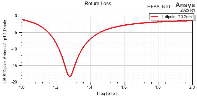
[10]:
spar_plot = hfss.create_scattering(plot="Return Loss", sweep=interp_sweep.name)
PyAEDT INFO: Parsing C:\Users\ansys\AppData\Local\Temp\tmpo3hnzd9r.ansys\dipole.aedt.
PyAEDT INFO: File C:\Users\ansys\AppData\Local\Temp\tmpo3hnzd9r.ansys\dipole.aedt correctly loaded. Elapsed time: 0m 0sec
PyAEDT INFO: aedt file load time 0.05626559257507324
PyAEDT INFO: PostProcessor class has been initialized! Elapsed time: 0m 0sec
PyAEDT INFO: PostProcessor class has been initialized! Elapsed time: 0m 0sec
PyAEDT INFO: Post class has been initialized! Elapsed time: 0m 0sec
Visualize far-field data#
Parameters passed to hfss.post.create_report() specify which quantities will be displayed in the HFSS design. Below you can see how parameters map from Python to the reporter in the AEDT user interface.
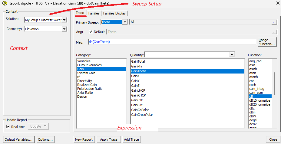
Note: These images were created using the 25R1 release.
[11]:
variations = hfss.available_variations.nominal_values
variations["Freq"] = [center_freq]
variations["Theta"] = ["All"]
variations["Phi"] = ["All"]
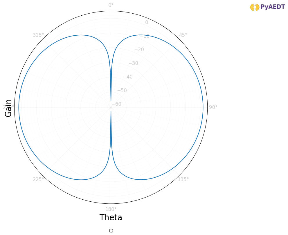
elevation_ffd_plot = hfss.post.create_report(
expressions="db(GainTheta)",
setup_sweep_name=disc_sweep.name,
variations=variations,
primary_sweep_variable="Theta",
context="Elevation", # Far-field setup is pre-defined.
report_category="Far Fields",
plot_type="Radiation Pattern",
plot_name="Elevation Gain (dB)",
)
elevation_ffd_plot.children["Legend"].properties["Show Trace Name"] = False
elevation_ffd_plot.children["Legend"].properties["Show Solution Name"] = False
Create a far-field report#
The hfss.post.reports_by_category helps simplify the syntax required to access post-processing capabilities. In this case, results are shown for the current variation. The concept of “variations” is essential for managing parametric solutions in HFSS.
The argument sphere_name specifies the far-field sphere used to generate the plot. In this case, the far-field sphere “3D” was automatically created when HFSS was launched by instantiating the Hfss class.
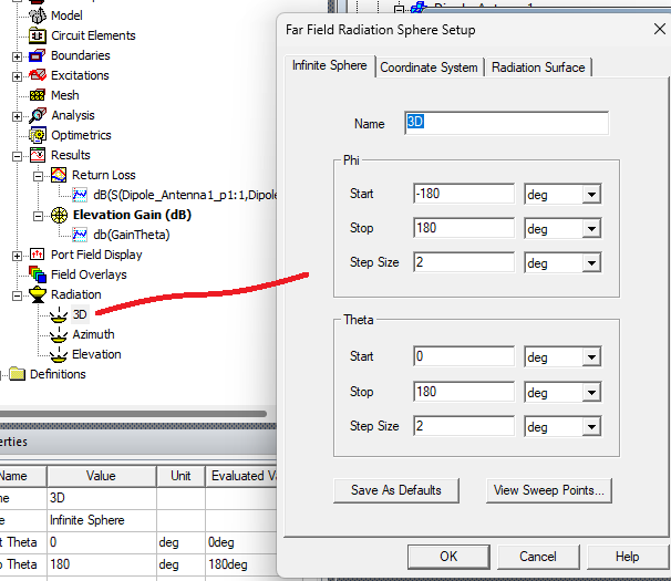
[12]:
report_3d = hfss.post.reports_by_category.far_field(
    "db(RealizedGainTheta)",
    disc_sweep.name,
    sphere_name="3D",
    Freq=[center_freq],
)

report_3d.report_type = "3D Polar Plot"
report_3d.create(name="Realized Gain (dB)")
[12]:
True
Retrieve far-field data for post-processing in Python#
Use the far-field visualizer to plot the realized gain and show the geometry. The far-field data is retrieved from HFSS and stored in a data class. The data class has a built-in method to generate the plot shown below.
[13]:
antenna_data = hfss.get_antenna_data(
    frequencies=[center_freq],
    setup=disc_sweep.name,
    sphere="3D",
)
new_plot = antenna_data.farfield_data.plot_3d(
    quantity="RealizedGain_Theta",
    quantity_format="dB10",
    output_file=os.path.join(hfss.working_directory, "Image.jpg"),
    show=False,
)
# ### View cross-polarization
#
# The dipole is linearly polarized as can be seen from the comparison of $\theta$-polarized
# and $\phi$-polarized "realized gain" at $\theta=90^\circ$ degrees.
# The following code creates the gain plots in AEDT.
PyAEDT INFO: Far field sphere 3D is assigned
PyAEDT INFO: Exporting antenna metadata...
PyAEDT INFO: Antenna metadata exported.
PyAEDT INFO: Exporting geometry...
C:\actions-runner\_work\pyaedt-examples\pyaedt-examples\.venv\lib\site-packages\ansys\aedt\core\visualization\plot\pyvista.py:1314: InvalidMeshWarning: PolyData mesh is not valid:
 - Mesh has 1 cell array with incorrect length (length must be 1). Invalid array: 'MaterialIds' (0)
  filedata = pv.read(cad.path)
PyAEDT INFO: Exporting embedded element patterns.... Done: 4.3971757888793945 seconds
C:\actions-runner\_work\pyaedt-examples\pyaedt-examples\.venv\lib\site-packages\ansys\aedt\core\visualization\plot\pyvista.py:1314: InvalidMeshWarning: PolyData mesh is not valid:
 - Mesh has 1 cell array with incorrect length (length must be 1). Invalid array: 'MaterialIds' (0)
  filedata = pv.read(cad.path)
WARNING:root:ERROR: In vtkDataSet.cxx, line 741
vtkPolyData (000002C5E6C13700): Cell array MaterialIds with 1 components, has only 0 tuples but there are 1 cells
WARNING:root:ERROR: In vtkDataSet.cxx, line 741
vtkPolyData (000002C5E6C12860): Cell array MaterialIds with 1 components, has only 0 tuples but there are 1 cells
WARNING:root:ERROR: In vtkDataSet.cxx, line 741
vtkPolyData (000002C5E6C13700): Cell array MaterialIds with 1 components, has only 0 tuples but there are 1 cells
WARNING:root:ERROR: In vtkDataSet.cxx, line 741
vtkPolyData (000002C5E6C12860): Cell array MaterialIds with 1 components, has only 0 tuples but there are 1 cells
[14]:
xpol_expressions = ["db(RealizedGainTheta)", "db(RealizedGainPhi)"]
xpol = hfss.post.reports_by_category.far_field(
    ["db(RealizedGainTheta)", "db(RealizedGainPhi)"],
    disc_sweep.name,
    name="Cross Polarization",
    sphere_name="Azimuth",
    Freq=[center_freq],
)

xpol.report_type = "Radiation Pattern"
xpol.create(name="xpol")
xpol.children["Legend"].properties["Show Solution Name"] = False
xpol.children["Legend"].properties["Show Variation Key"] = False
The get_solution_data() method is again used to create an inline plot of cross-polarization from the report in HFSS.
[15]:
ff_el_data = elevation_ffd_plot.get_solution_data()
_ = ff_el_data.plot(x_label="Theta", y_label="Gain", is_polar=True)
PyAEDT INFO: Solution Correctly loaded. Elapsed time: 0m 0sec
INFO:Global:Solution Correctly loaded. Elapsed time: 0m 0sec
PyAEDT INFO: Solution Correctly parsed. Elapsed time: 0m 0sec
INFO:Global:Solution Correctly parsed. Elapsed time: 0m 0sec
C:\actions-runner\_work\pyaedt-examples\pyaedt-examples\.venv\lib\site-packages\ansys\aedt\core\visualization\plot\matplotlib.py:1614: UserWarning: No artists with labels found to put in legend.  Note that artists whose label start with an underscore are ignored when legend() is called with no argument.
  self.legend = self.ax.legend(
Release AEDT#
[16]:
hfss.save_project()
hfss.release_desktop()

# Wait 3 seconds to allow AEDT to shut down before cleaning the temporary directory.
time.sleep(3)
PyAEDT INFO: Project dipole Saved correctly
INFO:Global:Project dipole Saved correctly
PyAEDT INFO: Desktop has been released and closed.
INFO:Global:Desktop has been released and closed.
Clean up#
All project files are saved in the folder temp_folder.name. If you’ve run this example as a Jupyter notebook, you can retrieve those project files. The following cell removes all temporary files, including the project folder.
[17]:
temp_folder.cleanup()
Download this example
Download this example as a Jupyter Notebook or as a Python script.